What are these meshfree modeling methods?

Spheral was conceived as a tool for the development and utilization of meshfree physics modeling algorithms, such as N-body gravitational models and Smoothed Particle Hydrodynamics (SPH). In order to understand how best to use Spheral and its applicability to a given problem, it is useful to have a basic grasp of how these sorts of meshfree methods work. This section is intended as a (very) brief introduction to these ideas – the interested researcher is encouraged to dive into the detailed references to gain a deeper understanding.

SPH began in the astrophysics community which was looking for a method of modeling hydrodynamics coupled with N-body gravity methods. Since N-body is particle based, it was natural to look for a hydrodynamics method which could also be particle based, and so SPH was born in the late 1970’s. SPH is indeed a method that solves the Lagrangian hydrodynamic conservation equations (mass, momentum, and energy) on points that move freely about the problem. Ordinary hydrodynamic methods usually discretize space using a mesh of some sort, which carves space up into cells. Meshfree methods instead distribute the mass of the problem amongst a finite number of points, which should be laid down conformally with the mass distribution being modeled. As an example, consider a 2D problem where we want represent a bounded circle of fluid using SPH:

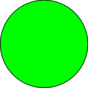A continuous fluid disk

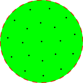Evenly spaced SPH nodes representing the fluid in this disk

Example of bounded circle of fluid in 2D we want to discretize using SPH

In this example we are representing the continuous green fluid on the left by evenly distributing a collection of SPH points in the volume of that fluid. Each of the SPH points carries the physics variables we need for the physics problem we’re trying to solve: mass, velocity, energy, temperature, deviatoric stress, etc. SPH like methods take a discrete representation from a finite number of points such as this and extend that to a continuous representation by convolving a so-called interpolation kernel over the values on these points. Interpolation kernels generally look like Gaussian functions of distance, except we generally use functions that have “compact support”, which simply means that these functions fall to zero and terminate at some finite distance from their central point (unlike Gaussians which are formally infinite). A cartoon representation of this interpolation process can be seen here:

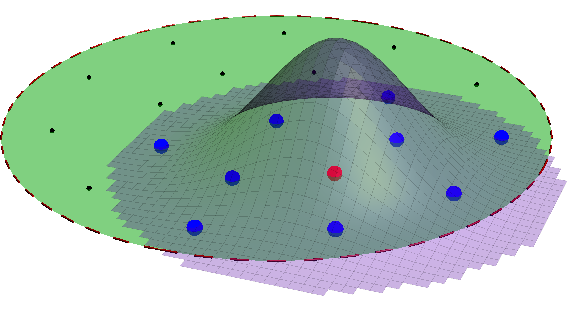
Notional SPH interpolation kernel centered on the red node. Blue node have non-zero values for the kernel, while the black points do not and therefore do not contribute to the state of the blue point in question. Here we are viewing the same notional 2D circular body of fluid from the previous figure, and the third dimension represents the magnitude of the kernel function for the red node.

In this example the interpolation kernel is centered on the red point, and has non-zero values extending over the blue points. However, it formally falls to zero outside this range, and therefore the black points do not contribute to the interpolation about the red point in question.

In SPH the interpolation kernel is represented by a function \(W(x^\alpha - x_i^\alpha, h)\) where \(x^\alpha - x_i^\alpha\) is the vector displacement between the sampling position and a point denoted by the index \(i\), and \(h\) is the so-called smoothing scale which has units of length. Most of the functions we use for interpolation kernels reduce to functions of the normalized distance \(W(\eta)\), where \(\eta^\alpha \equiv (x^\alpha - x_i^\alpha)/h\) is the dimensionless coordinate vector and \(\eta = (\eta^\alpha \eta^\alpha)^{1/2}\) is its magnitude.

Note

A note about notation in this guide. We use roman letter indices to represent the indices of specific points (so \(m_i\) is the mass of point \(i\)) and Greek indices to represent components of vectors and tensors (\(v_i^\alpha\) is the \(\alpha\)th component of the vector value \(\vec{v}_i\)). We also use the Einstein summation convention for repeated Greek indices, so \(\vec{a} \cdot \vec{b} \equiv a^\alpha b^\alpha\).

Common examples of functions that might be used as interpolation kernels include

• Gaussian: \(W(\eta) = A \exp(-\eta^2)\)

• Wendland C4: \(W(\eta) = A \left(1 - \eta\right)^6 \left(1 + 6 \eta + \frac{35}{3} \eta^2\right), \forall \; \eta \le 1\)

where the constant \(A\) is used to enforce a volume normalization on the integral of \(W\) such that \(\int W(\eta) \, dV = 1\). Using this convention we can represent this volume convolution for SPH interpolation for a spatial field \(F(x^\alpha)\) as

\[\begin{split}\langle F(x^\alpha) \rangle &= \int F({x^\prime}^\alpha) W({x^\prime}^\alpha - x^\alpha, h) dV \approx \sum_j V_j F(x_j^\alpha) W(x_j^\alpha - x^\alpha, h) \\ \langle \partial_\beta F(x^\alpha) \rangle &\approx \sum_j V_j F(x_j^\alpha) \partial_\beta W(x_j^\alpha - x^\alpha, h) \\\end{split}\]

In these relations we’ve transitioned from the continuous integral representations to the discrete numerical approximations represented by sums over particles (represented by the neighbor point indices \(j\)), which is the crux of how SPH works. In this discrete approximation SPH provides numerical estimates of fields and their spatial gradients at any point in space (most crucially at the interpolation points themselves). This same mathematical framework allows us to perform this spatial convolution over general partial differential equations (PDE’s) and arrive at numerical approximations for those PDE’s as simple sums over the points near a given particle as functions of the interpolation kernel. For instance, the following are standard SPH representations of the Lagrangian conservation relations for mass, momentum, and energy in the fluid regime:

\[\begin{split}\frac{D\rho}{Dt} &= -\rho \partial_\alpha v^\alpha \approx \rho_i \sum_j m_j (v_i^\alpha - v_j^\alpha) \partial_\alpha W_{ij} \\ \frac{Dv^\alpha}{Dt} &= -\rho^{-1} \partial_\alpha P \approx -\sum_j m_j \left( \frac{P_i}{\rho_i^2} + \frac{P_j}{\rho_j^2} \right) \partial_\alpha W_{ij} \\ \frac{D\varepsilon}{Dt} &= -\rho^{-1} P \partial_\alpha v^\alpha \approx -\frac{P_i}{\rho_i^2} \sum_j (v_i^\alpha - v_j^\alpha) \partial_\alpha W_{ij} \\\end{split}\]

or more generally in the solid regime including the full stress tensor (just the momentum and energy equations change):

\[\begin{split}\frac{Dv^\alpha}{Dt} &= \rho^{-1} \partial_\beta \sigma^{\alpha \beta} \approx \sum_j m_j \left( \rho_i^{-2} \sigma_i^{\alpha \beta} \partial_\beta W_i + \rho_j^{-2} \sigma_j^{\alpha \beta} \partial_\beta W_j \right) \\ \frac{D\varepsilon}{Dt} &= -\rho^{-1} \sigma^{\alpha \beta} \partial_\alpha v^\beta \approx -\sum_j m_j \rho_i^{-2} \sigma_i^{\alpha \beta} (v_i^\alpha - v_j^\alpha) \partial_\beta W_i \\\end{split}\]

where we have expressed these relations at a point \(i\) with position \(x_i^\alpha\), and the standard fluid variables are

\(\rho\)	mass density
\(V\)	volume
\(v^\alpha\)	velocity vector
\(P\)	pressure
\(\varepsilon\)	specific thermal energy
\(S^{\alpha \beta}\)	deviatoric stress
\(\sigma^{\alpha \beta} = S^{\alpha \beta} - P \delta^{\alpha \beta}\)	stress tensor

This leads us to a sometimes subtle but important distinction about these sorts of schemes: despite “Particle” being right there in the name of the method, SPH and its ilk are not really particle methods. The points in SPH are best viewed as moving centers of interpolation, on which we are solving partial differential equations (PDE’s), very similarly to how more traditional meshed methods such as finite-elements difference equation like these. For this reason in Spheral we use the term “nodes” rather than particles to refer to these moving interpolation points. This is in contrast to truly particle based numerical methods such as the discrete element method or molecular dynamics. We actually have a discrete element implementation available in Spheral as well, just to confuse the issue, so in those models our Spheral nodes really are best viewed as particles. But in the various fluid methods available in Spheral, such as SPH, CRKSPH (Conservative Reproducing Kernel SPH), or FSISPH (Fluid-Solid Interface SPH), it is worth keeping in mind this distinction in order to better understand the models and what their results mean.